Hybrid Classification & Embedding

In this example we’ll set up a hybrid ParaDime routine that can both classify high-dimensional data and embed it in a two dimensional space. Our routine will learn both tasks simultaneously with a shared latent space of the model.

We start by importing some packages and the relevant ParaDime submodules. We also call ParaDime’s seed utility for reproducibility reasons.

import copy
import torch
from matplotlib import pyplot as plt

import paradime.dr
import paradime.loss
import paradime.models
import paradime.routines
import paradime.utils

paradime.utils.seed.seed_all(42);

We test our hybrid model on the MNIST handwritten image dataset available via torchvision.

import torchvision

mnist = torchvision.datasets.MNIST(
    '../data',
    train=True,
    download=True,
)
mnist_data = mnist.data.reshape(-1, 28*28) / 255.
num_items = 5000

mnist_subset = mnist_data[:num_items]
target_subset = mnist.targets[:num_items]

Defining Our Custom Model

Let’s now define our hybrid model. In our model’s __init__ we simply create a list of fully connected layers depending on our input and hidden layer dimensions. From the final hidden layer, the model branches out into an embedding part with default dimensionality 2 and another part for classification, which depends on the number of target classes.

class HybridEmbeddingModel(paradime.models.Model):
    """A fully connected network for hybrid embedding and classification.

    Args:
        in_dim: Input dimension.
        hidden_dims: List of hidden layer dimensions.
        num_classes: Number of target classes.
        emb_dim: Embedding dimension (2 by default).
    """

    def __init__(self,
        in_dim: int,
        hidden_dims: list[int],
        num_classes: int,
        emb_dim: int = 2,
    ):
        super().__init__()

        self.layers = torch.nn.ModuleList()

        cur_dim = in_dim
        for hdim in hidden_dims:
            self.layers.append(torch.nn.Linear(cur_dim, hdim))
            cur_dim = hdim

        self.emb_layer = torch.nn.Linear(cur_dim, emb_dim)
        self.class_layer = torch.nn.Linear(cur_dim, num_classes)

        self.alpha = torch.nn.Parameter(torch.tensor(1.0))

    def common_forward(self, x):
        for layer in self.layers:
            # x = torch.sigmoid(layer(x))
            x = layer(x)
            x = torch.nn.functional.softplus(x)
        return x

    def embed(self, x):
        x = self.common_forward(x)
        x = self.emb_layer(x)
        return x

    def classify(self, x):
        x = self.common_forward(x)
        x = self.class_layer(x)
        return x

The model has a common_forward method, which propagates the input until the final hidden layer. It also has an embed method that takes the common forward output (i.e., latent representation) and embeds it, and a classify method that takes the same representation and turns it into prediction scores.

Defining the ParaDime Routine

Now we can define our ParaDime routine. We’ll borrow most settings from ParaDime’s built-in ParametricTSNE class.

To do this, we first define a dummy parametric TSNE routine:

tsne = paradime.routines.ParametricTSNE(in_dim=28*28)

Now we can acces our dummy method’s relations, training phases, and the main embedding loss:

global_rel = tsne.global_relations
batch_rel = tsne.batch_relations
init_phase, main_phase = tsne.training_phases
rel_loss = main_phase.loss

With these building blocks, we can go on to define our routine. In the following cell, quite a lot of things happen. Let’s break it down one by one:

• First we define a list of weights, which we will later use in a compound loss to run a bunch of experiments at once.

• Then we set up a dictionary of losses containing the original t-SNE loss and a simple classification loss. Because we implemented our custom model with a classify method, we don’t have to specify anything else in the classification loss.

• We’re ready to define our hybrid_tsne routine now. As a model we use our HybridEmbeddingModel. The rest of the settings are the ones we copied from the built-in class above.

• We add a training phase to the routine that uses both losses with the corresponding weights. To this end, we pass the respective settings to the loss_keys and loss_weights parameters.

• Finally, we can call the routine’s train method, making sure to supply the main data and the required class labels.

The three blocks of code that follow the training are just there for saving the embedded MNIST subsets and our classifier’s accuracies for each weight.

embeddings = []
train_accuracies = []
test_accuracies = []

weights = [0.0, 5.0, 20.0, 50.0, 100.0, 200.0, 300.0, 500.0]

losses = {"tsne": rel_loss, "class": paradime.loss.ClassificationLoss()}

for w in weights:

    paradime.utils.logging.log(f"Weight: {w}")

    hybrid_tsne = paradime.dr.ParametricDR(
        model=HybridEmbeddingModel(
            in_dim=28 * 28, hidden_dims=[100, 50], num_classes=10, emb_dim=2,
        ),
        global_relations=global_rel,
        batch_relations=batch_rel,
        losses=losses,
        use_cuda=True,
        verbose=True,
    )
    hybrid_tsne.add_training_phase(
        epochs=50,
        batch_size=500,
        learning_rate=0.001,
        loss_keys=["tsne", "class"],
        loss_weights=[w, 1.0],
    )
    hybrid_tsne.train({
        "main": mnist_subset,
        "labels": target_subset,
    })

    embeddings.append(hybrid_tsne.apply(mnist_subset, "embed"))

    train_logits = hybrid_tsne.apply(mnist_subset, "classify")
    train_prediction = torch.argmax(train_logits, dim=1)
    train_accuracies.append(
        torch.sum(train_prediction == target_subset) / num_items
    )

    test_logits = hybrid_tsne.apply(
        mnist_data[num_items : 2 * num_items], "classify"
    )
    test_prediction = torch.argmax(test_logits, dim=1)
    test_accuracies.append(
        torch.sum(test_prediction == mnist.targets[num_items : 2 * num_items])
        / num_items
    )

2022-12-05 17:35:57,037: Weight: 0.0
2022-12-05 17:35:57,053: Initializing training dataset.
2022-12-05 17:35:57,054: Computing global relations 'rel'.
2022-12-05 17:35:57,055: Indexing nearest neighbors.
2022-12-05 17:36:00,495: Calculating probabilities.
2022-12-05 17:36:00,899: Beginning training phase 'None'.
2022-12-05 17:36:01,524: Loss after epoch 0: 23.374043226242065
2022-12-05 17:36:04,791: Loss after epoch 5: 6.746389925479889
2022-12-05 17:36:07,537: Loss after epoch 10: 3.327723205089569
2022-12-05 17:36:10,121: Loss after epoch 15: 2.488990306854248
2022-12-05 17:36:12,493: Loss after epoch 20: 2.063904419541359
2022-12-05 17:36:14,884: Loss after epoch 25: 1.7633165121078491
2022-12-05 17:36:17,302: Loss after epoch 30: 1.5405211821198463
2022-12-05 17:36:19,748: Loss after epoch 35: 1.3202617168426514
2022-12-05 17:36:22,149: Loss after epoch 40: 1.1230880618095398
2022-12-05 17:36:24,618: Loss after epoch 45: 0.9901934340596199
2022-12-05 17:36:26,575: Weight: 5.0
2022-12-05 17:36:26,580: Initializing training dataset.
2022-12-05 17:36:26,581: Computing global relations 'rel'.
2022-12-05 17:36:26,582: Indexing nearest neighbors.
2022-12-05 17:36:29,849: Calculating probabilities.
2022-12-05 17:36:30,167: Beginning training phase 'None'.
2022-12-05 17:36:30,620: Loss after epoch 0: 23.421343326568604
2022-12-05 17:36:33,080: Loss after epoch 5: 6.376019656658173
2022-12-05 17:36:35,580: Loss after epoch 10: 3.552820473909378
2022-12-05 17:36:38,035: Loss after epoch 15: 2.923263341188431
2022-12-05 17:36:40,501: Loss after epoch 20: 2.568203628063202
2022-12-05 17:36:42,976: Loss after epoch 25: 2.2359817028045654
2022-12-05 17:36:45,682: Loss after epoch 30: 1.974912941455841
2022-12-05 17:36:48,192: Loss after epoch 35: 1.7780115008354187
2022-12-05 17:36:50,660: Loss after epoch 40: 1.5792310014367104
2022-12-05 17:36:53,165: Loss after epoch 45: 1.417787104845047
2022-12-05 17:36:55,177: Weight: 20.0
2022-12-05 17:36:55,183: Initializing training dataset.
2022-12-05 17:36:55,183: Computing global relations 'rel'.
2022-12-05 17:36:55,185: Indexing nearest neighbors.
2022-12-05 17:36:58,551: Calculating probabilities.
2022-12-05 17:36:58,923: Beginning training phase 'None'.
2022-12-05 17:36:59,390: Loss after epoch 0: 24.98308563232422
2022-12-05 17:37:02,164: Loss after epoch 5: 7.412625193595886
2022-12-05 17:37:04,747: Loss after epoch 10: 4.617538094520569
2022-12-05 17:37:07,434: Loss after epoch 15: 3.9158853590488434
2022-12-05 17:37:10,017: Loss after epoch 20: 3.5313377380371094
2022-12-05 17:37:12,615: Loss after epoch 25: 3.1707524359226227
2022-12-05 17:37:15,335: Loss after epoch 30: 2.9148961305618286
2022-12-05 17:37:17,814: Loss after epoch 35: 2.69510680437088
2022-12-05 17:37:20,375: Loss after epoch 40: 2.524357244372368
2022-12-05 17:37:22,911: Loss after epoch 45: 2.335147351026535
2022-12-05 17:37:24,993: Weight: 50.0
2022-12-05 17:37:24,999: Initializing training dataset.
2022-12-05 17:37:24,999: Computing global relations 'rel'.
2022-12-05 17:37:25,000: Indexing nearest neighbors.
2022-12-05 17:37:28,521: Calculating probabilities.
2022-12-05 17:37:28,881: Beginning training phase 'None'.
2022-12-05 17:37:29,379: Loss after epoch 0: 27.679900646209717
2022-12-05 17:37:31,885: Loss after epoch 5: 9.593429267406464
2022-12-05 17:37:34,549: Loss after epoch 10: 6.798569738864899
2022-12-05 17:37:37,182: Loss after epoch 15: 6.045582473278046
2022-12-05 17:37:39,679: Loss after epoch 20: 5.615615129470825
2022-12-05 17:37:42,226: Loss after epoch 25: 5.385365605354309
2022-12-05 17:37:44,752: Loss after epoch 30: 5.036754310131073
2022-12-05 17:37:47,265: Loss after epoch 35: 4.851190388202667
2022-12-05 17:37:49,898: Loss after epoch 40: 4.612240374088287
2022-12-05 17:37:52,480: Loss after epoch 45: 4.394551336765289
2022-12-05 17:37:54,630: Weight: 100.0
2022-12-05 17:37:54,634: Initializing training dataset.
2022-12-05 17:37:54,634: Computing global relations 'rel'.
2022-12-05 17:37:54,636: Indexing nearest neighbors.
2022-12-05 17:37:58,155: Calculating probabilities.
2022-12-05 17:37:58,479: Beginning training phase 'None'.
2022-12-05 17:37:58,968: Loss after epoch 0: 32.28746175765991
2022-12-05 17:38:01,513: Loss after epoch 5: 13.215462446212769
2022-12-05 17:38:04,116: Loss after epoch 10: 10.221698343753815
2022-12-05 17:38:06,921: Loss after epoch 15: 9.45009845495224
2022-12-05 17:38:10,260: Loss after epoch 20: 8.906982719898224
2022-12-05 17:38:12,995: Loss after epoch 25: 8.523437321186066
2022-12-05 17:38:15,537: Loss after epoch 30: 8.197549939155579
2022-12-05 17:38:18,101: Loss after epoch 35: 7.991234600543976
2022-12-05 17:38:20,640: Loss after epoch 40: 7.6662933230400085
2022-12-05 17:38:23,259: Loss after epoch 45: 7.479751467704773
2022-12-05 17:38:25,379: Weight: 200.0
2022-12-05 17:38:25,384: Initializing training dataset.
2022-12-05 17:38:25,385: Computing global relations 'rel'.
2022-12-05 17:38:25,386: Indexing nearest neighbors.
2022-12-05 17:38:28,871: Calculating probabilities.
2022-12-05 17:38:29,233: Beginning training phase 'None'.
2022-12-05 17:38:29,730: Loss after epoch 0: 42.272467613220215
2022-12-05 17:38:32,234: Loss after epoch 5: 20.484930515289307
2022-12-05 17:38:34,854: Loss after epoch 10: 16.981189489364624
2022-12-05 17:38:37,434: Loss after epoch 15: 15.911800861358643
2022-12-05 17:38:40,062: Loss after epoch 20: 15.33408260345459
2022-12-05 17:38:42,610: Loss after epoch 25: 14.829533696174622
2022-12-05 17:38:45,218: Loss after epoch 30: 14.510748386383057
2022-12-05 17:38:47,772: Loss after epoch 35: 14.062031269073486
2022-12-05 17:38:50,337: Loss after epoch 40: 13.682900547981262
2022-12-05 17:38:53,083: Loss after epoch 45: 13.267605543136597
2022-12-05 17:38:55,194: Weight: 300.0
2022-12-05 17:38:55,198: Initializing training dataset.
2022-12-05 17:38:55,199: Computing global relations 'rel'.
2022-12-05 17:38:55,200: Indexing nearest neighbors.
2022-12-05 17:38:58,747: Calculating probabilities.
2022-12-05 17:38:59,072: Beginning training phase 'None'.
2022-12-05 17:38:59,575: Loss after epoch 0: 51.94435501098633
2022-12-05 17:39:02,209: Loss after epoch 5: 26.590487003326416
2022-12-05 17:39:04,788: Loss after epoch 10: 23.415546894073486
2022-12-05 17:39:07,398: Loss after epoch 15: 22.646225929260254
2022-12-05 17:39:10,052: Loss after epoch 20: 21.6688050031662
2022-12-05 17:39:12,718: Loss after epoch 25: 20.953031182289124
2022-12-05 17:39:16,127: Loss after epoch 30: 20.51979398727417
2022-12-05 17:39:19,178: Loss after epoch 35: 19.985873579978943
2022-12-05 17:39:21,912: Loss after epoch 40: 19.605836272239685
2022-12-05 17:39:24,563: Loss after epoch 45: 19.279836893081665
2022-12-05 17:39:26,608: Weight: 500.0
2022-12-05 17:39:26,611: Initializing training dataset.
2022-12-05 17:39:26,612: Computing global relations 'rel'.
2022-12-05 17:39:26,613: Indexing nearest neighbors.
2022-12-05 17:39:30,174: Calculating probabilities.
2022-12-05 17:39:30,580: Beginning training phase 'None'.
2022-12-05 17:39:31,052: Loss after epoch 0: 71.35737419128418
2022-12-05 17:39:33,649: Loss after epoch 5: 41.27285051345825
2022-12-05 17:39:36,251: Loss after epoch 10: 37.69342231750488
2022-12-05 17:39:38,788: Loss after epoch 15: 35.554267168045044
2022-12-05 17:39:41,325: Loss after epoch 20: 34.69854784011841
2022-12-05 17:39:43,846: Loss after epoch 25: 33.6288857460022
2022-12-05 17:39:46,403: Loss after epoch 30: 32.77002167701721
2022-12-05 17:39:49,158: Loss after epoch 35: 32.27752494812012
2022-12-05 17:39:51,723: Loss after epoch 40: 31.387125968933105
2022-12-05 17:39:54,248: Loss after epoch 45: 30.70688772201538

Plotting the Results

Once the training has completed (which might take while, since we train 8 different routines from scratch), we can take a look at the results.

ParaDime’s scatterplot utility function accepts an ax keyword parameter. We can create a grid of Matplotlib axes and, in a loop, pass each axis as ax to create the scatterplot inside the grid. To the final grid cell we add a plot of the accuracies as a function of the losses’ weights:

fig = plt.figure(figsize=(15, 15))

for i, (emb, w) in enumerate(zip(embeddings, weights)):
    ax = fig.add_subplot(3, 3, i + 1)

    paradime.utils.plotting.scatterplot(
        emb,
        labels=target_subset,
        ax=ax,
        legend=(i == 0),
        legend_options={"loc": 3},
    )
    ax.set_title(f"w_emb / w_class = {w}")

palette = paradime.utils.plotting.get_color_palette()
ax = fig.add_subplot(3, 3, 9)
ax.plot(weights, train_accuracies, c=palette["petrol"])
ax.plot(weights, test_accuracies, c=palette["aqua"])
ax.set_xscale("log")
ax.set_ylim([0,1])
ax.legend(["train", "test"])
ax.set_title("Classification accuracy");

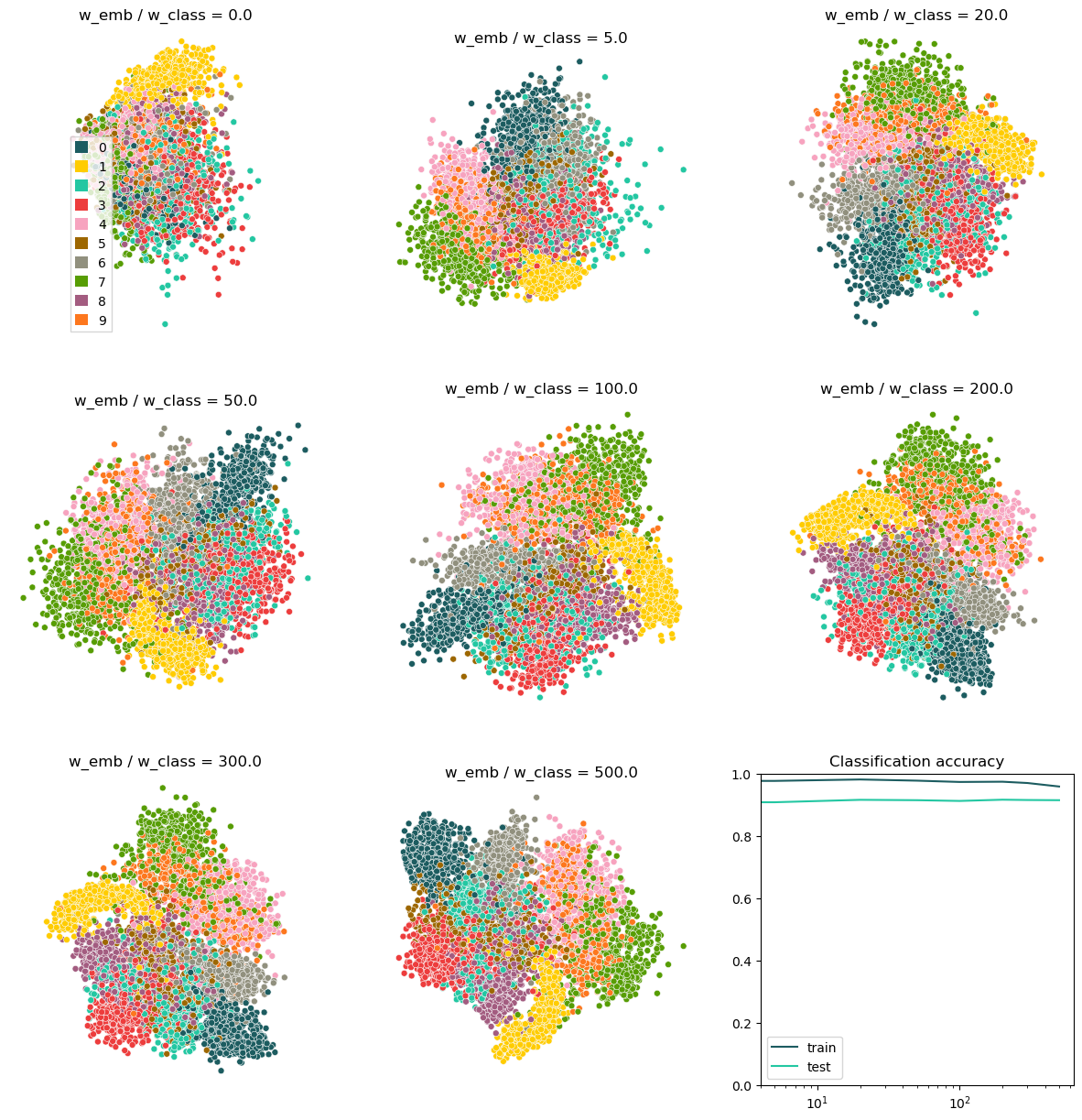
The plot in the top left corner shows the embedding of the latent space for pure classification. While the embedding function is random here (because the embedding branch of our model was not trained at all), we can still see some clusters because our model has learned to group classes together in the latent space. With increasing weight on the embedding loss, the plot starts to look more like we would expect a t-SNE of MNIST to look like. Despite this, the classification accuracy remains high, as cen be seen in the accuracy plot on the bottom right. Only for very high weights of the embedding loss, the train accuracy drops. Interetingly though, the test accuracy ramains stable (maybe even increasing ever so slightly). This means that the strong focus on embedding does not hurt the classifier to generalize at all.

In summary, we have succesfully trained a model that can perform both tasks, classification and t-SNE-like embedding, pretty well.