Guiding Embeddings by Correlation

This example is very similar to the Supervised DR example. There, we definde a triplet loss that was based on the class labels. Here, we are going to define a loss that constrains the embedding based on one of the original, high-dimensional data attributes. In particular, we will make one of the embedding coordinates correlate with one selected data attribute.

Data Preprocessing

First we will set up our training data. This part is the same as in the Supervised DR example.

import numpy as np
import torch
import sklearn.datasets
import sklearn.decomposition
import sklearn.manifold
import sklearn.preprocessing
from matplotlib import pyplot as plt

import paradime.dr
import paradime.relations
import paradime.transforms
import paradime.loss
import paradime.utils

paradime.utils.seed.seed_all(42);

covertype = sklearn.datasets.fetch_covtype()

label_to_name = {
    1: "Spruce/fir",
    2: "Lodgepole pine",
    3: "Ponderosa pine",
    4: "Cottonwood/willow",
    5: "Aspen",
    6: "Douglas-fir",
    7: "Krummholz",
}

_, counts = np.unique(covertype.target, return_counts=True)
weights = np.array([ 1/counts[i-1] for i in covertype.target ])

indices = list(torch.utils.data.WeightedRandomSampler(weights, 7000))

raw_data = covertype.data[indices,:10]
scaler = sklearn.preprocessing.StandardScaler()
scaler.fit(raw_data)
data = scaler.transform(raw_data)

Relations and Derived Data

Now we set up the relations and the derived data entry necessary for PCA initialization. Again, this part is exactly the same as in the Supervised DR example.

tsne_global_rel = paradime.relations.NeighborBasedPDist(
    transform=[
        paradime.transforms.PerplexityBasedRescale(
            perplexity=200, bracket=[0.001, 1000]
        ),
        paradime.transforms.Symmetrize(),
        paradime.transforms.Normalize(),
    ]
)

tsne_batch_rel = paradime.relations.DifferentiablePDist(
    transform=[
        paradime.transforms.StudentTTransform(alpha=1.0),
        paradime.transforms.Normalize(),
        paradime.transforms.ToSquareTensor(),
    ]
)

def pca(x):
    return sklearn.decomposition.PCA(n_components=2).fit_transform(x)

derived = paradime.dr.DerivedData(pca)

Custom Loss

We can now define the correlation-based custom loss. The Loss has a forward function that expects a certain call signature. We simply select the respective dimensions of the low- and high-dimensional data and compute the correlation between them.

class GuidingLoss(paradime.loss.Loss):
    """Triplet loss for supervised DR.

    This loss constrains an embedding in such a way that the specified
    dimension of the embedding correlates with the specified high-dimensional
    data attribute.

    Args:
        attr_index: The index of the high-dimensional data attribute.
        emb_dim: The index of the embedding dimension.
    """

    def __init__(self, attr_index, emb_dim, data_key="main", name=None):
        super().__init__(name)

        self.attr_index = attr_index
        self.emb_dim = emb_dim
        self.data_key = data_key

    def forward(self, model, global_relations, batch_relations, batch, device):

        data = batch[self.data_key].to(device)
        emb = model.embed(data)

        chosen_attr = data[:, self.attr_index]
        chosen_emb_coord = emb[:, self.emb_dim]

        # the following lines implement Pearson's correlation coefficient
        # in a differentiable way

        cov = torch.cov(
            torch.stack((chosen_attr, chosen_emb_coord))
        )

        corr = cov[0,1] / (chosen_attr.std() * chosen_emb_coord.std())

        # the actual loss is 1 minus the squared correlation

        loss = 1 - corr**2

        return loss

Setting up the Routine

We can now set up the routine in the same way as we did in the Supervised DR example. We just define a dict of all our losses and combine them by passing several loss_keys to the embedding training phase.

In this example we make the x-coordinate of the embedding (index 0) correlate with the “Hillshade (noon)” attribute of the data (index 7).

losses = {
    "init": paradime.loss.PositionLoss(position_key="pca"),
    "embedding": paradime.loss.RelationLoss(
        loss_function=paradime.loss.kullback_leibler_div,
    ),
    "guiding": GuidingLoss(7, 0),
}

We then set up training phases for the PCA initialization and for the actual embedding. In this example we are going to train multiple routines with different weights on the losses. To make things easier, we define a function that sets up the guided embedding phase for us.

tsne_init = paradime.dr.TrainingPhase(
    name="pca_init",
    loss_keys=["init"],
    batch_size=500,
    epochs=10,
    learning_rate=0.01,
)

def guided_phase(w):

    weights = [w if w != -1 else 1, 1 if w != -1 else 0]

    return paradime.dr.TrainingPhase(
        name="embedding",
        loss_keys=["embedding", "guiding"],
        loss_weights=weights,
        batch_size=500,
        epochs=40,
        learning_rate=0.02,
        report_interval=2,
)

Now we can run our experiment for a given set of weights:

weights = [-1, 5000, 1000, 100]
routines = []

for w in weights:
    super_tsne = paradime.dr.ParametricDR(
        global_relations=tsne_global_rel,
        batch_relations=tsne_batch_rel,
        derived_data={"pca": derived},
        losses=losses,
        in_dim=10,
        out_dim=2,
        hidden_dims=[100, 50],
        use_cuda=True,
        verbose=True,
    )
    super_tsne.add_training_phase(tsne_init)
    super_tsne.add_training_phase(guided_phase(w))
    super_tsne.train(data)

    routines.append(super_tsne)

2022-12-05 16:17:02,044: Initializing training dataset.
2022-12-05 16:17:02,046: Computing derived data entry 'pca'.
2022-12-05 16:17:02,061: Adding entry 'pca' to dataset.
2022-12-05 16:17:02,063: Computing global relations 'rel'.
2022-12-05 16:17:02,064: Indexing nearest neighbors.
2022-12-05 16:17:32,098: Calculating probabilities.
2022-12-05 16:17:33,613: Beginning training phase 'pca_init'.
2022-12-05 16:17:35,198: Loss after epoch 0: 11.940744780004025
2022-12-05 16:17:35,582: Loss after epoch 5: 0.014664343849290162
2022-12-05 16:17:36,051: Beginning training phase 'embedding'.
2022-12-05 16:17:38,762: Loss after epoch 0: 0.05023368517868221
2022-12-05 16:17:44,476: Loss after epoch 2: 0.04354730644263327
2022-12-05 16:17:50,155: Loss after epoch 4: 0.04269229085184634
2022-12-05 16:17:55,923: Loss after epoch 6: 0.042116038501262665
2022-12-05 16:18:01,720: Loss after epoch 8: 0.041533354902639985
2022-12-05 16:18:07,597: Loss after epoch 10: 0.04116497584618628
2022-12-05 16:18:13,468: Loss after epoch 12: 0.040755698224529624
2022-12-05 16:18:19,407: Loss after epoch 14: 0.0405914313159883
2022-12-05 16:18:25,342: Loss after epoch 16: 0.040183454751968384
2022-12-05 16:18:31,326: Loss after epoch 18: 0.04015950602479279
2022-12-05 16:18:37,362: Loss after epoch 20: 0.04008115897886455
2022-12-05 16:18:43,365: Loss after epoch 22: 0.03993109078146517
2022-12-05 16:18:49,396: Loss after epoch 24: 0.03963697864674032
2022-12-05 16:18:55,488: Loss after epoch 26: 0.039588446263223886
2022-12-05 16:19:01,551: Loss after epoch 28: 0.03957401495426893
2022-12-05 16:19:07,719: Loss after epoch 30: 0.03940155799500644
2022-12-05 16:19:13,798: Loss after epoch 32: 0.039539771154522896
2022-12-05 16:19:19,936: Loss after epoch 34: 0.03946721274405718
2022-12-05 16:19:26,045: Loss after epoch 36: 0.039164590649306774
2022-12-05 16:19:32,115: Loss after epoch 38: 0.0393480584025383
2022-12-05 16:19:35,176: Initializing training dataset.
2022-12-05 16:19:35,177: Computing derived data entry 'pca'.
2022-12-05 16:19:35,187: Adding entry 'pca' to dataset.
2022-12-05 16:19:35,188: Computing global relations 'rel'.
2022-12-05 16:19:35,188: Indexing nearest neighbors.
2022-12-05 16:19:50,757: Calculating probabilities.
2022-12-05 16:19:51,950: Beginning training phase 'pca_init'.
2022-12-05 16:19:52,058: Loss after epoch 0: 18.271042108535767
2022-12-05 16:19:52,445: Loss after epoch 5: 0.017542065063025802
2022-12-05 16:19:52,759: Beginning training phase 'embedding'.
2022-12-05 16:19:55,760: Loss after epoch 0: 258.91400718688965
2022-12-05 16:20:01,885: Loss after epoch 2: 227.05931854248047
2022-12-05 16:20:08,035: Loss after epoch 4: 223.05237483978271
2022-12-05 16:20:14,115: Loss after epoch 6: 218.14965724945068
2022-12-05 16:20:20,822: Loss after epoch 8: 215.3008394241333
2022-12-05 16:20:27,586: Loss after epoch 10: 215.72983741760254
2022-12-05 16:20:34,163: Loss after epoch 12: 211.0892629623413
2022-12-05 16:20:40,468: Loss after epoch 14: 212.2063045501709
2022-12-05 16:20:46,662: Loss after epoch 16: 211.31444454193115
2022-12-05 16:20:52,925: Loss after epoch 18: 210.32128429412842
2022-12-05 16:20:59,182: Loss after epoch 20: 209.44341564178467
2022-12-05 16:21:05,444: Loss after epoch 22: 207.95620918273926
2022-12-05 16:21:11,706: Loss after epoch 24: 207.25160026550293
2022-12-05 16:21:17,925: Loss after epoch 26: 204.96608066558838
2022-12-05 16:21:24,140: Loss after epoch 28: 205.60664463043213
2022-12-05 16:21:30,402: Loss after epoch 30: 206.29371070861816
2022-12-05 16:21:36,617: Loss after epoch 32: 205.9644021987915
2022-12-05 16:21:42,918: Loss after epoch 34: 206.93801879882812
2022-12-05 16:21:49,192: Loss after epoch 36: 204.23660373687744
2022-12-05 16:21:55,389: Loss after epoch 38: 204.68682670593262
2022-12-05 16:21:58,516: Initializing training dataset.
2022-12-05 16:21:58,517: Computing derived data entry 'pca'.
2022-12-05 16:21:58,532: Adding entry 'pca' to dataset.
2022-12-05 16:21:58,534: Computing global relations 'rel'.
2022-12-05 16:21:58,535: Indexing nearest neighbors.
2022-12-05 16:22:14,804: Calculating probabilities.
2022-12-05 16:22:15,958: Beginning training phase 'pca_init'.
2022-12-05 16:22:16,041: Loss after epoch 0: 10.833057437092066
2022-12-05 16:22:16,439: Loss after epoch 5: 0.014823349076323211
2022-12-05 16:22:16,769: Beginning training phase 'embedding'.
2022-12-05 16:22:19,780: Loss after epoch 0: 56.204397439956665
2022-12-05 16:22:25,939: Loss after epoch 2: 51.61842370033264
2022-12-05 16:22:32,193: Loss after epoch 4: 50.38016128540039
2022-12-05 16:22:38,436: Loss after epoch 6: 49.956124782562256
2022-12-05 16:22:44,778: Loss after epoch 8: 49.45035362243652
2022-12-05 16:22:51,144: Loss after epoch 10: 48.82789421081543
2022-12-05 16:22:57,411: Loss after epoch 12: 48.2091224193573
2022-12-05 16:23:03,731: Loss after epoch 14: 48.346463203430176
2022-12-05 16:23:10,016: Loss after epoch 16: 48.153064012527466
2022-12-05 16:23:16,288: Loss after epoch 18: 47.62262797355652
2022-12-05 16:23:22,584: Loss after epoch 20: 47.46352934837341
2022-12-05 16:23:28,859: Loss after epoch 22: 47.20341515541077
2022-12-05 16:23:35,139: Loss after epoch 24: 47.10884714126587
2022-12-05 16:23:41,434: Loss after epoch 26: 46.94178223609924
2022-12-05 16:23:47,722: Loss after epoch 28: 46.588475942611694
2022-12-05 16:23:53,955: Loss after epoch 30: 46.933860540390015
2022-12-05 16:24:00,276: Loss after epoch 32: 46.707542419433594
2022-12-05 16:24:06,566: Loss after epoch 34: 46.57085061073303
2022-12-05 16:24:12,844: Loss after epoch 36: 46.389081716537476
2022-12-05 16:24:19,161: Loss after epoch 38: 46.105255126953125
2022-12-05 16:24:22,279: Initializing training dataset.
2022-12-05 16:24:22,280: Computing derived data entry 'pca'.
2022-12-05 16:24:22,290: Adding entry 'pca' to dataset.
2022-12-05 16:24:22,292: Computing global relations 'rel'.
2022-12-05 16:24:22,293: Indexing nearest neighbors.
2022-12-05 16:24:38,918: Calculating probabilities.
2022-12-05 16:24:40,095: Beginning training phase 'pca_init'.
2022-12-05 16:24:40,179: Loss after epoch 0: 11.92252480238676
2022-12-05 16:24:40,741: Loss after epoch 5: 0.010523691569687799
2022-12-05 16:24:41,059: Beginning training phase 'embedding'.
2022-12-05 16:24:44,212: Loss after epoch 0: 6.978371351957321
2022-12-05 16:24:50,572: Loss after epoch 2: 5.372454285621643
2022-12-05 16:24:56,792: Loss after epoch 4: 5.2515000104904175
2022-12-05 16:25:03,082: Loss after epoch 6: 5.170226126909256
2022-12-05 16:25:09,331: Loss after epoch 8: 5.086310476064682
2022-12-05 16:25:15,599: Loss after epoch 10: 5.0369886457920074
2022-12-05 16:25:21,865: Loss after epoch 12: 5.005982846021652
2022-12-05 16:25:28,172: Loss after epoch 14: 4.982121556997299
2022-12-05 16:25:34,416: Loss after epoch 16: 4.9463100135326385
2022-12-05 16:25:40,740: Loss after epoch 18: 4.906199663877487
2022-12-05 16:25:47,010: Loss after epoch 20: 4.867999821901321
2022-12-05 16:25:53,256: Loss after epoch 22: 4.88426598906517
2022-12-05 16:25:59,697: Loss after epoch 24: 4.864299476146698
2022-12-05 16:26:06,036: Loss after epoch 26: 4.802669733762741
2022-12-05 16:26:12,322: Loss after epoch 28: 4.799461632966995
2022-12-05 16:26:18,578: Loss after epoch 30: 4.826367110013962
2022-12-05 16:26:24,920: Loss after epoch 32: 4.750685662031174
2022-12-05 16:26:31,204: Loss after epoch 34: 4.739946216344833
2022-12-05 16:26:37,457: Loss after epoch 36: 4.7596370577812195
2022-12-05 16:26:43,767: Loss after epoch 38: 4.739692151546478

Visualizing the Results

Let’s now visualize the results and see how the correlation loss affects the embedding. This time, we’ll color the scatterplot by the data attribute that we chose for our loss (hillshade at noon).

fig = plt.figure(figsize=(20,5))
for i, r in enumerate(routines):
    ax = fig.add_subplot(1,len(routines), i + 1)
    # ax.set_title(weights[j])
    paradime.utils.plotting.scatterplot(
        r.apply(data),
        c=data[:,7],
        cmap=paradime.utils.plotting.get_colormap(),
        ax=ax,
    )
fig.subplots_adjust(wspace=0)

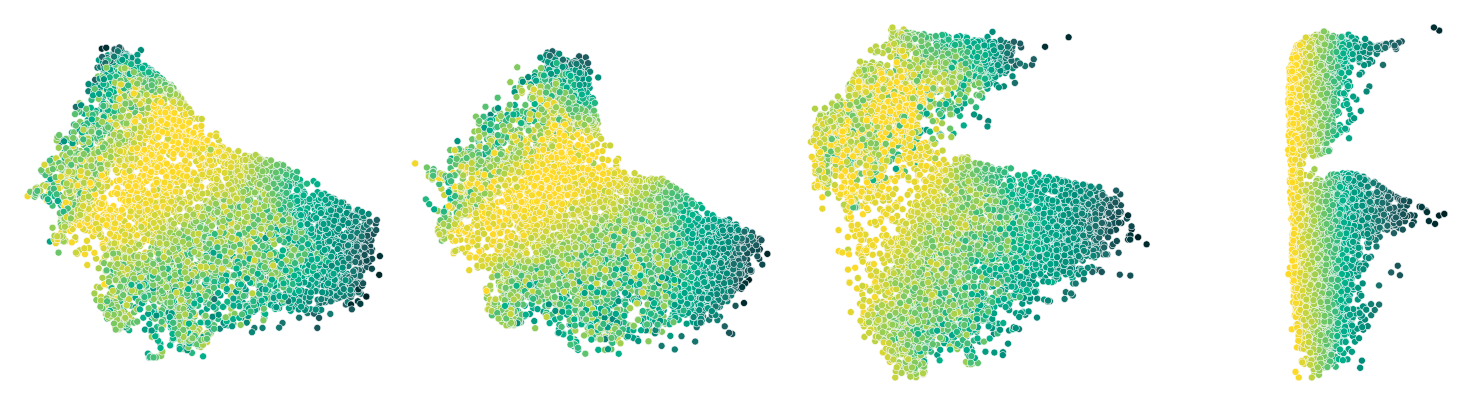
Note how with the increasing weight on the new guiding loss, the embedding is gradually morphed in such a way that our chosen attribute changes smoothly from left to right.

Verifying the Feature Importance

As a final step, we’ll verify that the selected feature has in fact become more important for the x-axis of our embedding. We’ll also investigate what happened to the y-axis.

To do this, we can apply a simple version of integrated gradients. Since all ParaDime routines are based on a neural network, we can apply any model-agnostic or NN-specific explainability methods to it. The integrated-gradient-based estimate for the feature importance that we use here is just a basic example of what can be done.

Let’s first compute the gradients for the completely unguided routine:

unguided = routines[0]

grads_x_unguided = []
grads_y_unguided = []

for d in data:
    unguided.model.forward(torch.tensor(d).float().cuda())[0].backward()
    grads_x_unguided.append(unguided.model.layers[0].weight.grad.sum(dim=0))
    unguided.model.zero_grad()

    unguided.model.forward(torch.tensor(d).float().cuda())[1].backward()
    grads_y_unguided.append(unguided.model.layers[0].weight.grad.sum(dim=0))
    unguided.model.zero_grad()

grads_x_unguided = torch.stack(grads_x_unguided).cpu()
grads_y_unguided = torch.stack(grads_y_unguided).cpu()

Now we do the same for the most strongly guided routine:

guided = routines[-1]

grads_x_guided = []
grads_y_guided = []

for d in data:
    guided.model.forward(torch.tensor(d).float().cuda())[0].backward()
    grads_x_guided.append(guided.model.layers[0].weight.grad.sum(dim=0))
    guided.model.zero_grad()

    guided.model.forward(torch.tensor(d).float().cuda())[1].backward()
    grads_y_guided.append(guided.model.layers[0].weight.grad.sum(dim=0))
    guided.model.zero_grad()

grads_x_guided = torch.stack(grads_x_guided).cpu()
grads_y_guided = torch.stack(grads_y_guided).cpu()

We can now assemble the data in a data frame:

import pandas as pd

feature_names = [ str(i) for i in np.arange(1, 11) ]

guided_total_x = grads_x_guided.mean(dim=0).abs().sum()
guided_total_y = grads_y_guided.mean(dim=0).abs().sum()
unguided_total_x = grads_x_unguided.mean(dim=0).abs().sum()
unguided_total_y = grads_y_unguided.mean(dim=0).abs().sum()

df = pd.DataFrame()
df["Importance"] = np.concatenate(
    (
        grads_x_guided.flatten() / guided_total_x,
        grads_y_guided.flatten() / guided_total_y,
        grads_x_unguided.flatten() / unguided_total_x,
        grads_y_unguided.flatten() / unguided_total_y,
    )
)
df["Feature"] = np.tile(np.tile(feature_names, len(grads_x_guided)), 4)
df["Axis"] = np.tile(
    np.repeat(["x", "y"], len(grads_x_guided) * len(feature_names)), 2
)
df["Guided"] = np.repeat(
    [True, False], 2 * len(grads_x_guided) * len(feature_names)
)

Finally, we use seaborn to plot a bar chart that shows the aggregated gradient data:

import seaborn as sns

fig, (ax1, ax2) = plt.subplots(2, 1, figsize=(3, 7))

pd_palette = paradime.utils.plotting.get_color_palette()
palette = [pd_palette["petrol"], "lightgrey"]

sns.barplot(
    data=df[~df["Guided"]],
    y="Feature",
    x="Importance",
    hue="Axis",
    palette=palette,
    estimator=lambda x: abs(np.mean(x)),
    ci=None,
    ax=ax1,
)
ax1.set_xlabel("")
ax1.set_xticklabels("")
ax1.set_xlim(0, 0.35)
ax1.text(0.33, 9.0, "Unguided", ha="right")

sns.barplot(
    data=df[df["Guided"]],
    y="Feature",
    x="Importance",
    hue="Axis",
    palette=palette,
    estimator=lambda x: abs(np.mean(x)),
    ci=None,
    ax=ax2,
)
ax2.legend()
ax2.set_xlabel("Relative importance")
ax2.set_xlim(0, 0.35)

ax2.legend([],[], frameon=False)
ax2.text(0.33, 9.0, "Guided", ha="right")

fig.subplots_adjust(hspace=0.1)

fig.savefig("guided-bar.pdf", bbox_inches = "tight")

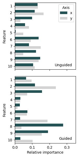
From these bar charts we can indeed conclude that the feature importance of the selected feature has increased substantially for the x-axis, but not changed much for the y-axis.